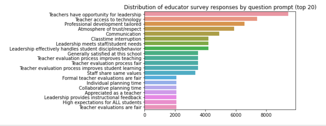
In continued pursuit to answer the question “Why are teachers changing schools frequently or leaving the classroom altogether?”, the Tennessee Educator Survey data is examined for evidence of one of the environmental microsystems defined in the previous statistical analysis.

The findings of the statistical analysis show that teachers across the state of Tennessee are closely divided in their feelings about their work environment. Those who feel positively barely outnumber those who feel negatively on any given metric.

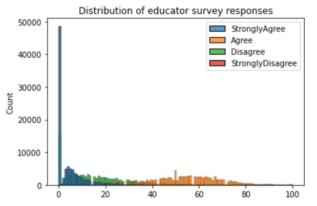
0 response represents a single unanswered question in an otherwise completed survey

While immediate steps can be taken to address educator’s top concerns statewide to make Tennessee schools more positive work environments overall, we continue to address our analysis of this issue by examining an environmental issue on a local level as a named step toward building a national model.

As discussed in our statistical analysis, teachers do not control their environment. They have influence in their classrooms and the relationships they build with student families and peers.

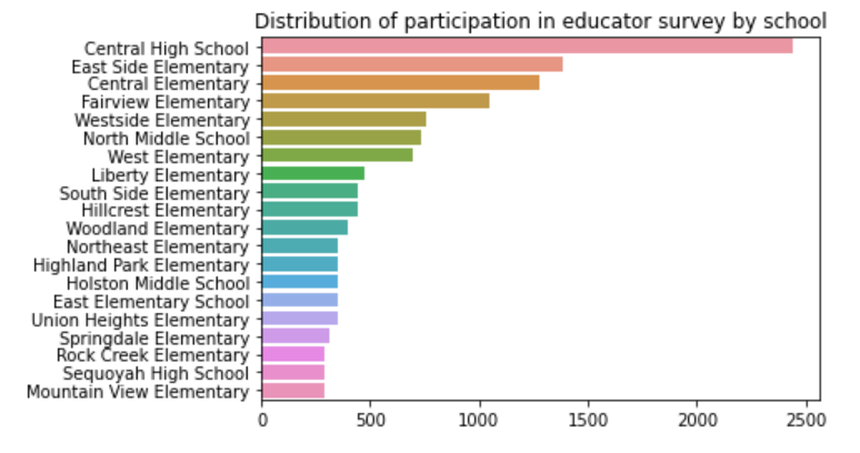
The question we now address “Is the way a teacher feels about their work environment correlated to the type of school (or district) in which they work?”.

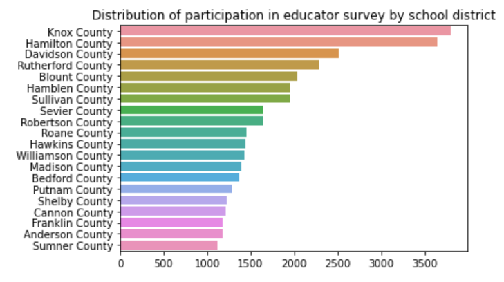
The type of school defines the community it serves as the classifier which determines public policy and state and federal funding for that school (and/or district).

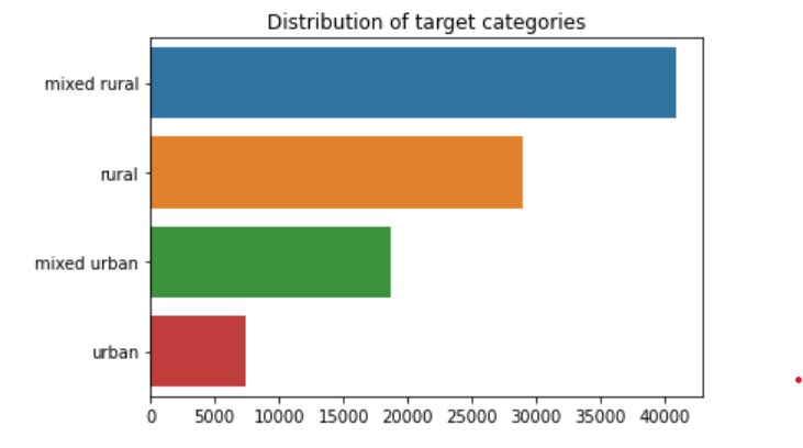
By creating and implementing machine learning statistical and classification models, we are able to analyze results from the annual Tennessee Educator Survey to determine if teacher responses are able predict the type of school in which a teacher is employed: urban, mixed urban, mixed rural, or rural.
This value is our predictive ‘target’.

The Process

Preprocessing

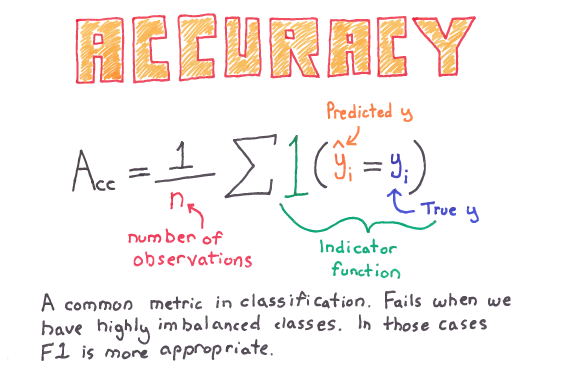
In order to evaluate categorical features, which our target value is, we must use the value counts method for baseline accuracy of our classification model. As we move into our model we will compare this value with accuracy and accuracy score.

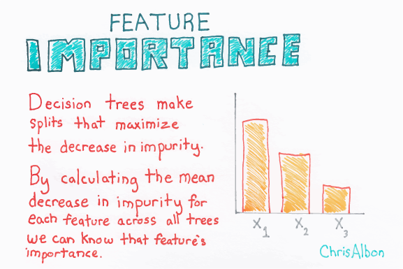
Feature importance and selection plays such an import role in our model because we are using a tree model (Random Forest Classifier) that splits and maximizes the decrease in impurity. By calculating a features importance in relation to the target, we can select and pass to our model those features that will help our model generalize to new data and predict with both accuracy and precision.

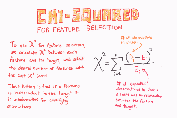
As proven through the Chi2 hypothesis testing, this dataset is highly relational. We will continue to use Chi2 for feature importance selection, to determine the exact nature of the relationship our numeric features have with our target variable and to determine how many features are optimal to include in our classification model.

While Chi2 is used to evaluate relationships between numeric features and the target, mutual information classification is used to evaluate relationships between categorical features and the target. Since half of our dataset is numeric and half categorical. We must use both processes to address leakage in the entire dataset.

Transformers in Python can be used to clean, reduce, expand or generate features. The fit method learns parameters from a training set and the transform method applies transformations to unseen data.

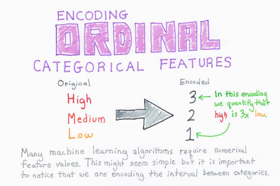
During preprocessing, we use several of Sci-Kit Learn’s transformers to prepare features to pass through the models. Label Encoder allows us to transform non-numeric data found in the target to numeric values. The Ordinal Encoder does the same thing for all other features.

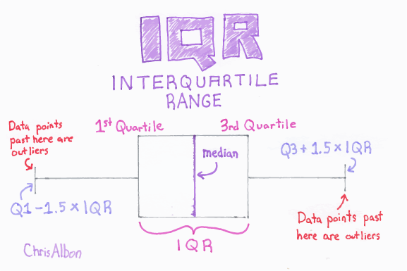
Robust Scaler centers the data by removing the median and scaling the data along the interquartile range. This standardizes the data and removes outliers.

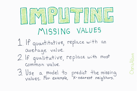
Most datasets contain missing values, represented by NaNs or other placeholders. They may even be encoded as blank values. Machine learning models cannot process missing values. Any observations (rows) or features (columns) in a dataset that are made up of entirely missing values are dropped from the dataset. However, it would be very costly (in information) to drop all observations and features that are simply incomplete. Simple Imputer fills in the missing values with the median.

Each of the describe transformers pre-process features in a different manner that allows data to pass through a pipeline and be fit to a machine learning model.

Algorithms

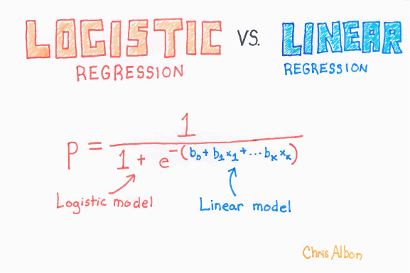
Logistic regression is a supervised learning classification algorithm used to predict the probability of a target variable. The nature of the target or dependent variable is dichotomous, which means there would be only two possible classes. In our model, the hyperparameter “solver” is set to “saga” in order to accommodate the large size of the dataset while claiming fewer computational penalties. Because our dataset has much higher cardinality than two, we have marginal results with this first level classifier.

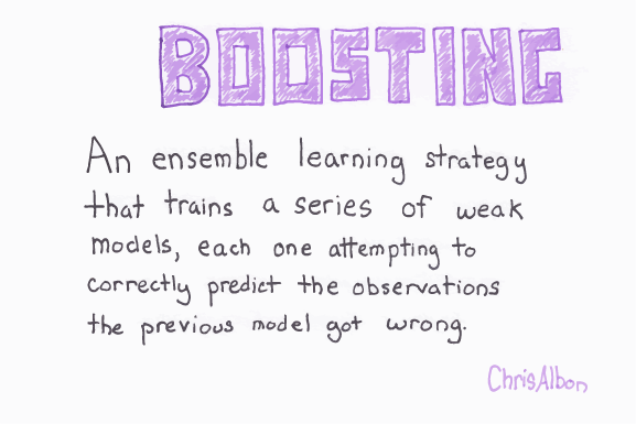
In order to get more from our dataset, we next use a classifier similar to ADABoost but works better with gradient descent. After adjusting the hyperparameters of the XGBoost Classifier, our model accuracy more than doubles.

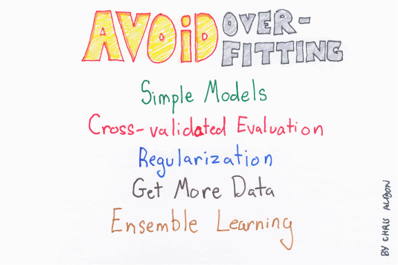
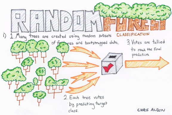
To avoid overfitting, we pass our data through the final algorithm, a random forest classifier. The random forest classifier uses averaging to help improve accuracy in a model and reduce overfitting. Unlike XGCBoost, random forest is not very sensitive to hyperparameter manipulation. However, we do set the hyperparameter “criterion” to “entropy” for information gain.

Metrics

Below are the reported metrics for our model throughout the development process:

For Baseline Accuracy we used the value counts method for classification.

 Baseline Accuracy: 0.42803702543758915

We compare Baseline Accuracy with Accuracy Score for the Logistic Regression model for classification. The Accuracy Score tells us how well (how accurately) our model predicts the target values.

 Training Accuracy, predicted values, logistic regression:  0.4289069840275603
 Validation Accuracy, predicted values, logistic regression:  0.4303460514640639

The low training and validation accuracy scores tells us that the Logistic Regression algorithm is not the best model for a multiple classification problem. Even so, this is a good place to start. Our model can only become more accurate from here. We add the XGCBoost algorithm to our model.

Next we compare our previous Accuracy Score with the Score for the XGCBoost algorithm for classification. The Score tells us how well (how accurately) our model predicts the target values.

 Training Accuracy: XGboost 0.9307860945818979
 Validation Accuracy: XGboost 0.9244219426901196

The XGCBoost algorith more than doubled our models predictive accuracy. However, in order to avoid overfitting the model, we continue to build our model by adding the Random Forest Classifier algoritm to our Model.

Next we compare our XGCBoost Score with the Accuracy Score for the Random Random Forest Classifier algorithm. The Accuracy Score tells us how well (how accurately) our model predicts the target values.

 Training Accuracy: random forest model 0.946775933465567
 Validation Accuracy: random forest model 0.8717052038206587
 Testing Accuracy: random forest model:  0.8795281344607997

The Accuracy Scores for the Random Forest Classifier seem to be well generalized to the data on the surface. To validate the acutal accuracy of our models ability to generalize to new data, we will use the K-Fold Cross-Validation method where k=3.

 train: [    0     2     3 ... 95787 95789 95790], test: [    1     4     6 ... 95784 95785 95788]
 train: [    0     1     4 ... 95788 95789 95790], test: [    2     3    11 ... 95781 95782 95787]
 train: [    1     2     3 ... 95785 95787 95788], test: [    0     5     7 ... 95786 95789 95790]

The metric Cross Validation Score validates our model is able to use educator survey responses to generalize to new data and predict the type of school an educator works in with an average of 95.78% accuracy.

Summary Vizualizations

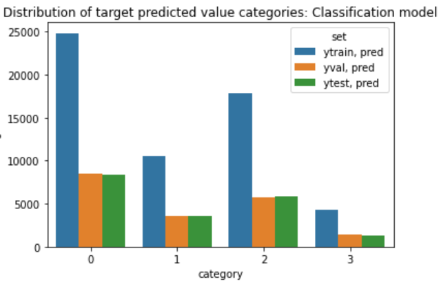
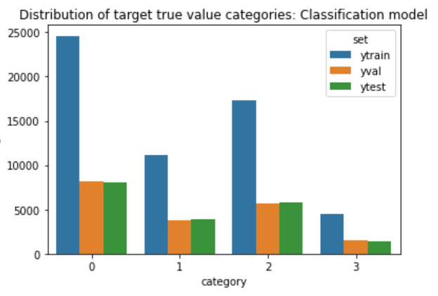
As a final check, call it a common sense test or a gut check, we visual map the results of the the distribution of the true values and then the predicted values. We see the distributions are extremely close. This is in alignment with our statistical results.

Conclusion

Combining the metrics visualualizations validation we conclude that our model can use educator survey responses to accurately predict the type of school an educator teaches in. Now we know that whether a teacher works in an urban, mixed urban, mixed rural, or rural environment has a high correlation to whether or not an enducator feels their working environment is positive or negative.

A closer analysis of the impact on teaching in each of these environments is needed as we continued to discover why teachers are leaving the classroom.

Sources:

Albon, Chris. Machine Learning Flashcards

Tennessee Advisory Commission on Intergovernmental Relations (TACIR), 2016. Just How Rural or Urban are Tennessee’s 95 Counties?

**

Additional Resources:

leakage: https://arxiv.org/abs/2001.10648

pipeline: https://machinelearningmastery.com/automate-machine-learning-workflows-pipelines-python-scikit-learn/

gradient descent: https://towardsdatascience.com/implement-gradient-descent-in-python-9b93ed7108d1

overfitting: https://docs.aws.amazon.com/machine-learning/latest/dg/model-fit-underfitting-vs-overfitting.html

information gain: https://towardsdatascience.com/gini-index-vs-information-entropy-7a7e4fed3fcb

**

And don’t forget…

…to keep Digging into the data!!

RJProctor, Data Scientist, MEd